Abstract
To design the linear accelerators and to make the particle tracking simulations a rf-gap model for the accelerating cells has to be implemented. The standard rectangular rf-gap field presentation, as well the trapezium and cos-like waveform field models were analyzed and compared.
INTRODUCTION
For
the accelerator design (mainly for linear accelerators [1]) an influence of the
accelerating elements on the transverse and longitudinal particle dynamics is
an important part to create a rf-gap
model. Further the general rf-gap mathematical
description is based on the paper [1], where the longitudinal particle dynamics
is characterized by:
- an average electric field on the axis of the
accelerating period
![]() , (1)
, (1)
where ![]() is an acceleration
period length;
is an acceleration
period length; ![]() is a waveform factor of
the axis electric field,
is a waveform factor of
the axis electric field, ![]() is the
longitudinal coordinate;
is the
longitudinal coordinate;
- the time flight coefficient
![]() ; (2)
; (2)
- the synchronous particle rf-phase
at the gap center ![]() .
.
The standard model for the transverse rf-gap action uses the matrix presentation [1,2], consisting from the thin lens matrices for the edge rf-gap electric field and a matrix for the rf-gap central part (as a rule the drift space matrix).
Note, the further results were got for the accelerating elements
of the ion linear accelerators, where a particle energy increase is much less
then the particle energy.
TRANSVERSE PRESENTATION
Supposing
the azimuthally symmetric gap electromagnetic field and neglecting by the
particle displacement along the rf-gap, the particle
trajectory refractions in the input and output gap halves will be [1]
![]() (3)
(3)
![]() ,
,
where ![]() ;
; ![]() is the angular rf-field frequency;
is the angular rf-field frequency; ![]() is the transverse
particle displacement;
is the transverse
particle displacement; ![]() and
and ![]() are the charge and
mass of the accelerating particles;
are the charge and
mass of the accelerating particles; ![]() is the light speed;
is the light speed; ![]() is the longitudinal
particle velocity;
is the longitudinal
particle velocity; ![]() is the particle relativistic
factor;
is the particle relativistic
factor; ![]() ;
; ![]() and
and ![]() are the first and
second rf-gap halves. Further the longitudinal
coordinate of the gap center will be defined as zero. The gap length is
are the first and
second rf-gap halves. Further the longitudinal
coordinate of the gap center will be defined as zero. The gap length is ![]() .
.
Trapezium rf-Gap Field
Waveform
The rf-field waveform is described by
 (4)
(4)
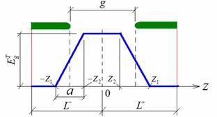
Figure 1: Trapezium rf-field waveform
The waveform (4) and some important parameters
are presented schematically in fig.1.
Substituting
(4) to (3), the followed expressions may be obtained
![]() (5)
(5)
![]() ,
,
where ![]() and
and ![]() are the synchronous
particle parameters at the gap center;
are the synchronous
particle parameters at the gap center; ![]() and
and ![]() are the average over
are the average over ![]() and
and ![]() coefficients
respectively;
coefficients
respectively; ![]() ;
; ![]() ;
; ![]() ;
; ![]() . The thin lenses (5) are placed in the points
. The thin lenses (5) are placed in the points
![]() .
.
Rectangular rf-Gap Field
Waveform
The
traditional representation of the rf-gap waveform is
a rectangular model:
![]() . (6)
. (6)
From (5) by assuming ![]() it follows
it follows
![]() (7)
(7)
![]() .
.
Cos-like rf-Gap Field
Waveform
The cos-like rf-field waveform is
described by
The thin lens refractions (3) will be
![]()
![]() , (9)
, (9)
where ![]() and
and ![]() .
.
LONGITUDINAL PRESENTATION
Assume
that there are some reliable estimations for the integral parameters (1) and
(2) (further they will be denoted ![]() and
and ![]() ) as well as for a gap coefficient
) as well as for a gap coefficient ![]() . Also there is the law to change the synchronous particle phase
. Also there is the law to change the synchronous particle phase ![]() . The longitudinal phase space coordinates
. The longitudinal phase space coordinates ![]() and an independent
time variable
and an independent
time variable ![]() will be used. The
synchronous particle transverse momentum is equal zero. The longitudinal
dynamics of the synchronous particle [1] is governed by
will be used. The
synchronous particle transverse momentum is equal zero. The longitudinal
dynamics of the synchronous particle [1] is governed by
![]()
![]() , (10)
, (10)
where ![]() is a rf-field phase of the
synchronous particle at the gap entrance. The rf-field
model is designed to conserve both the average electric field and time flight
coefficient the same as for the real rf-field (
is a rf-field phase of the
synchronous particle at the gap entrance. The rf-field
model is designed to conserve both the average electric field and time flight
coefficient the same as for the real rf-field (![]() and
and ![]() ).
).
Trapezium rf-Gap Field
Waveform
Applying the definitions and results of
the previous section the followed expressions may be derived:
![]() ,
, ![]() . (11)
. (11)
Therefore
![]() . (12)
. (12)
To define
the parameters ![]() it needs to solve
equation
it needs to solve
equation
![]() , (13)
, (13)
where ![]() . (14)
. (14)
As a rule
the practical values are ![]() and
and ![]() . However from (13) it follows the lowest limit to use the
proposed algorithm:
. However from (13) it follows the lowest limit to use the
proposed algorithm:
![]()
![]()
![]() . (15)
. (15)
To overcome the restriction (15) it was introduced the effective parameters
![]() . (16)
. (16)
As a result, ![]() and the parameter
and the parameter ![]() in (14) may be
increased up to the desired value, then the parameters
in (14) may be
increased up to the desired value, then the parameters ![]() and
and ![]() may be recalculated
according to (12). To solve the equation (13) the simple tangent method was
used. Finally all parameters of the trapezium rf-field
waveform (fig.1) will be determined with the requirements
may be recalculated
according to (12). To solve the equation (13) the simple tangent method was
used. Finally all parameters of the trapezium rf-field
waveform (fig.1) will be determined with the requirements
![]() and
and ![]() . (17)
. (17)
Rectangular rf-Gap
Field Waveform
Following
the approach from the above section and applying the field waveform (6) it may
be shown:
![]() ,
, ![]() (18)
(18)
![]() . (19)
. (19)
In practice for the real parameters the
inequality ![]() is always valid.
Therefore it was proposed to use the effective parameters
is always valid.
Therefore it was proposed to use the effective parameters
![]() ;
; ![]() . (20)
. (20)
As results it is possible to achieve the followed relations:
![]()
![]()
![]() . (21)
. (21)
Cos-like rf-Gap Field
Waveform
Following
the above approach the next relations may be derived:
![]() ,
,  (22)
(22)
![]() . (23)
. (23)
To defined
the parameter ![]() it needs to solve the
equation
it needs to solve the
equation
 , (24)
where all parameters are identical to ones in (14).
As a rule the practical values are ![]() and
and ![]() . However from (24) it follows the lowest limit to use the proposed
algorithm:
. However from (24) it follows the lowest limit to use the proposed
algorithm:
![]() . (25)
. (25)
The requirement (25) is more difficult compared with (15). Therefore the effective parameter approach is more probable for the cos-like rf-field waveform model. The formulas (16) are also valid. Finally all parameters of the waveform will be determined with the requirements
![]() ;
; ![]() . (26)
. (26)
PRACTICAL REALIZATION
The above mathematical models were realized to design qualitatively the accelerating elements of the ion linear accelerators. The proposed simulation algorithm consists from the followed stages:
·
the proposal of the specific parameters
of the accelerating structure : ![]() ,
, ![]() ,
, ![]() , the input velocity
, the input velocity ![]() and rf-phase
and rf-phase ![]() of the synchronous particle as well as the rf-phases of the synchronous particle at the gap center
of the synchronous particle as well as the rf-phases of the synchronous particle at the gap center ![]() and exit
and exit ![]() ;
;
·
the choice of the preliminary
gap geometry and rf-field waveform model, calculation
of the model characteristic parameters ![]() and
and ![]() ;
;
·
the simulation of the
synchronous particle dynamics (10) to get the synchronous particle phases at
the gap center ![]() and end
and end ![]() ;
;
·
applying the gradient method
and varying the ![]() and
and ![]() with conservation of
the
with conservation of
the ![]() ,
, ![]() ,
, ![]() to achieve the
equalities
to achieve the
equalities ![]() and
and ![]() ;
;
· in dependence from the rf-field waveform model to calculate the focusing properties (3) of the accelerating gap in the thin lens approximation.
The important integral parameter of the accelerating gap is the synchronous particle energy increase [1]:
![]() . (27)
. (27)
Excluding
the calculated gap length ![]() , all other parameters in (27) are identical for any applied rf-field waveform model. The value
, all other parameters in (27) are identical for any applied rf-field waveform model. The value ![]() is the result of the
computations presented above and therefore depends from the used rf-field waveform model.
is the result of the
computations presented above and therefore depends from the used rf-field waveform model.
To compare the studied models the calculations for Alvarez-type accelerating gap [3] were done. Additionally the simulation of the gap electromagnetic field was carried out by the power program codes [4]. The gap parameters were:
![]() cm ;
cm ;
![]() MHz
MHz
![]() MV/m ;
MV/m ;
![]() .
.
The graphical results are presented in fig.2, where the solid line is the data received by [4]; the dashed lines are the results for the different rf-field waveform models. The
highest rectangle was calculated by
using the rectangular model with the gap size ![]() whereas the lower rectangular is for the model with
whereas the lower rectangular is for the model with ![]() .
.
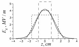
Figure 2: Computational rf-field waveform.
It is evidence the application of the trapezium and cos-like rf-field waveform models is more adequate to the real field distribution. The calculated parameters for the rf-gap are presented in Table 1. The cos-like rf-field waveform model has length the same as for the model with real rf-field distribution, thus the energy increase (27) for these models will be equal.
CONCLUSIONS
The various rf-field waveform models for the accelerating gap have been studied. It was shown that the cos-like rf-field waveform model is more adequate to the real field parameters compared with trapezium and rectangular waveform models. The developed algorithm is used both to design the ion linear accelerators and to study the multi particle dynamics of the accelerated beams.